library(dplyr)
library(ggplot2)
library(rstan)
library(lubridate)

options(mc.cores = parallel::detectCores())
rstan_options(auto_write = TRUE)

batting <- readRDS("data/batting.rds")
Introduction
James (Jimmy) Anderson is well known as one of the best ever pace bowlers to have played the game. His record speaks for itself - the most ever caps for an English test cricketer, the most ever wickets for a fast bowler in the history of test cricket, the only player to take 1000 first class wickets in the 21st century. Whilst he is known for his bowling achievements, in this article I will take a look at his batting throughout his test career.
His test career spans over 18 years, making his debut in May 2003 and still playing as of current (July 2021). For the duration of his career, it’s fair to say that batting has not been his strong point - he has usually been found at number 11 in the order. That’s not to say he’s an awful batsman, we’ve seen far worse batsmen during his career; when he and Monty Panesar were playing in the same team he would usually be given a promotion up to number 10. And despite the plethora of bowling records, he has a few batting records to go with it: he has the 5th most innings in test cricket before a duck, and he has the 3rd highest score by a number 11.
This article will be quite technical. I will be using the R programming language throughout, initially to perform some exploratory data analysis, and then later to create and compare mathematical models. These models are necessary so that we can understand how his batting has changed over time.
Exploratory Data Analysis
Firstly let’s take a glimpse at the data that we have.
batting %>% head(10)# A tibble: 10 × 4
innings_no date score dismissed
<int> <date> <dbl> <lgl>
1 1 2003-05-22 4 FALSE
2 2 2003-06-05 12 FALSE
3 3 2003-07-24 0 FALSE
4 4 2003-07-31 21 FALSE
5 5 2003-07-31 4 FALSE
6 6 2003-08-14 0 FALSE
7 7 2003-08-14 2 TRUE
8 8 2003-08-21 0 FALSE
9 9 2003-08-21 0 FALSE
10 10 2003-09-04 0 FALSE So we can see that we have the innings number, the date, the score and whether or not he was dismissed for each innings in test cricket that Jimmy Anderson has played.
To begin our analysis let’s plot the distribution of Jimmy’s batting scores.
batting %>%
  ggplot(aes(x = score, fill = dismissed)) +
  geom_bar() +
  scale_fill_discrete(name = "Dismissed?") +
  scale_x_continuous(name = "Score") +
  scale_y_continuous(name = "Count")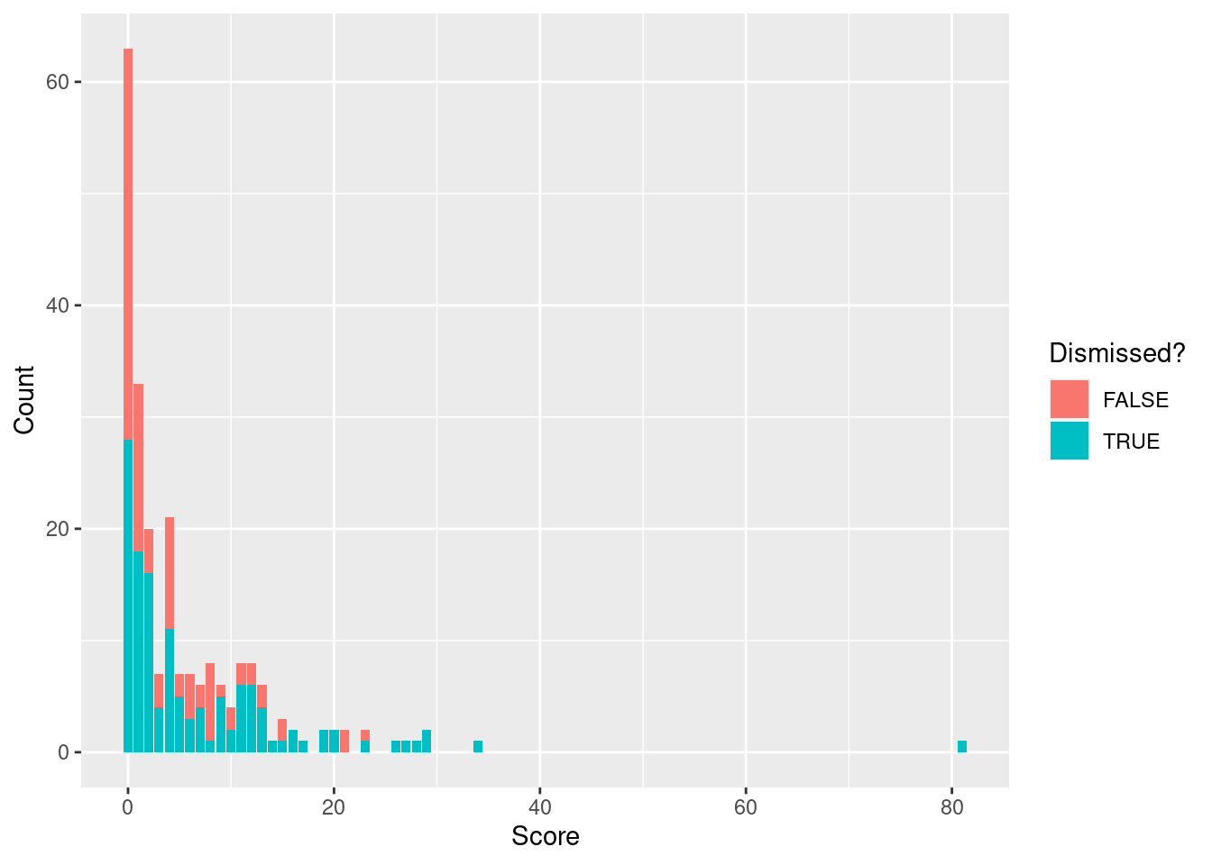
So despite not scoring a single duck (that is zero runs and out) in his first 54 innings, it is now his highest score when he is out. The scores look to follow a fairly geometric shape - this seems reasonable because you can think of a player having a constant probability of being dismissed before they score another run. Obviously this assumption does have some issues - you can see that Jimmy has been out for a score of 4 more often than a score of 3, and this is because scoring 4 runs through a single shot is quite common.
We are interested in how his batting has changed over time, so let’s plot his batting scores against the innings number.
batting %>%
  ggplot(aes(x = innings_no, y = score, col = dismissed)) +
  geom_point() +
  scale_y_continuous(breaks = seq(0, 90, by = 10), minor_breaks = NULL, name = "Score") +
  scale_x_continuous(name = "Innings Number") +
  scale_color_discrete(name = "Dismissed?")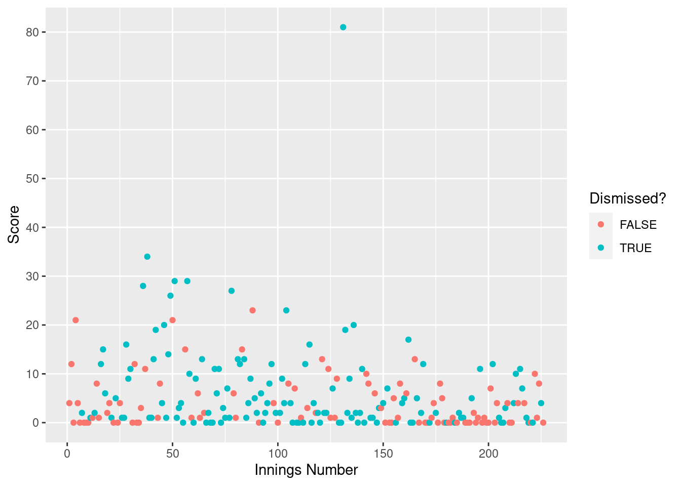
We can see that magnificent 81 at Trent Bridge in 2014 he scored standing out about half way through his career.
Colloquially, it is said that Jimmy’s batting has deteriorated over time. This excellent video by Jarrod Kimber explains how his batting, particularly against pace bowlers, has deteriorated as he has got older (and how he now only has one scoring shot which is the reverse sweep). The graph above supports that this is the case - just look at the number of times he passes 10 and larger scores in the first half of his career compared to more recently.
Whilst this graph has a lot of data points and therefore has a lot of variance meaning it can be difficult to see any patterns, lets cluster the data to see if that adds clarity. Lets start by looking at his batting average by year.
batting %>%
  group_by(year = year(date)) %>%
  summarise(
    ave = sum(score) / sum(dismissed)
  ) %>%
  ggplot(aes(x = year, y = ave)) +
  geom_point() +
  scale_x_continuous(name = "Year") +
  scale_y_continuous(name = "Batting Average")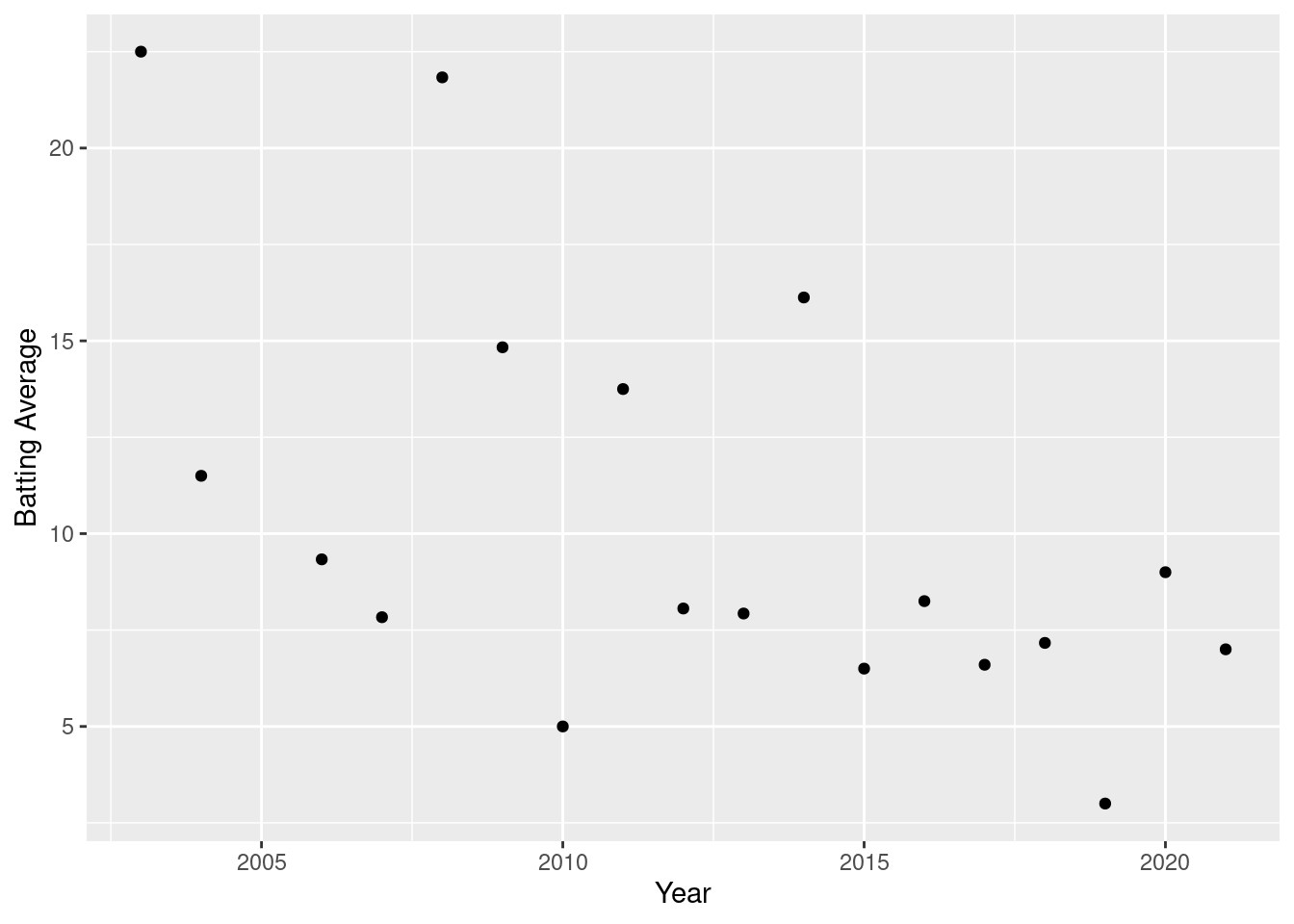
Whilst at first it might not again be initially obvious that there is clear pattern, we can see that Jimmy Anderson has averaged over 10 in 6 of his 18 calendar years (he didn’t play a game in 2005) as a professional cricketer, and the most recent of these was in 2014. So he hasn’t averaged over 10 in any of the past 7 years, but he averaged more than 10 in 4 of his first 7 years.
Let’s look into this further by calculating the rolling batting average for Anderson, where we take the nearest 25 innings either side to calculate this.
block_size <- 25
moving_batting_ave_df <- tibble(
  innings_no = numeric(),
  ave = numeric()
)
for (i in (block_size + 1):(nrow(batting) - block_size)) {
  moving_batting_ave <- batting %>%
    filter(
      innings_no >= i - block_size,
      innings_no <= i + block_size
    ) %>%
    summarise(ave = sum(score) / sum(dismissed)) %>%
    pull(ave)
  moving_batting_ave_df <- moving_batting_ave_df %>%
    add_row(
      innings_no = i,
      ave = moving_batting_ave
    )
}
moving_batting_ave_df %>%
  ggplot(aes(x = innings_no, y = ave)) +
  geom_point() +
  scale_x_continuous(name = "Innings Number") +
  scale_y_continuous(name = "Moving Batting Average")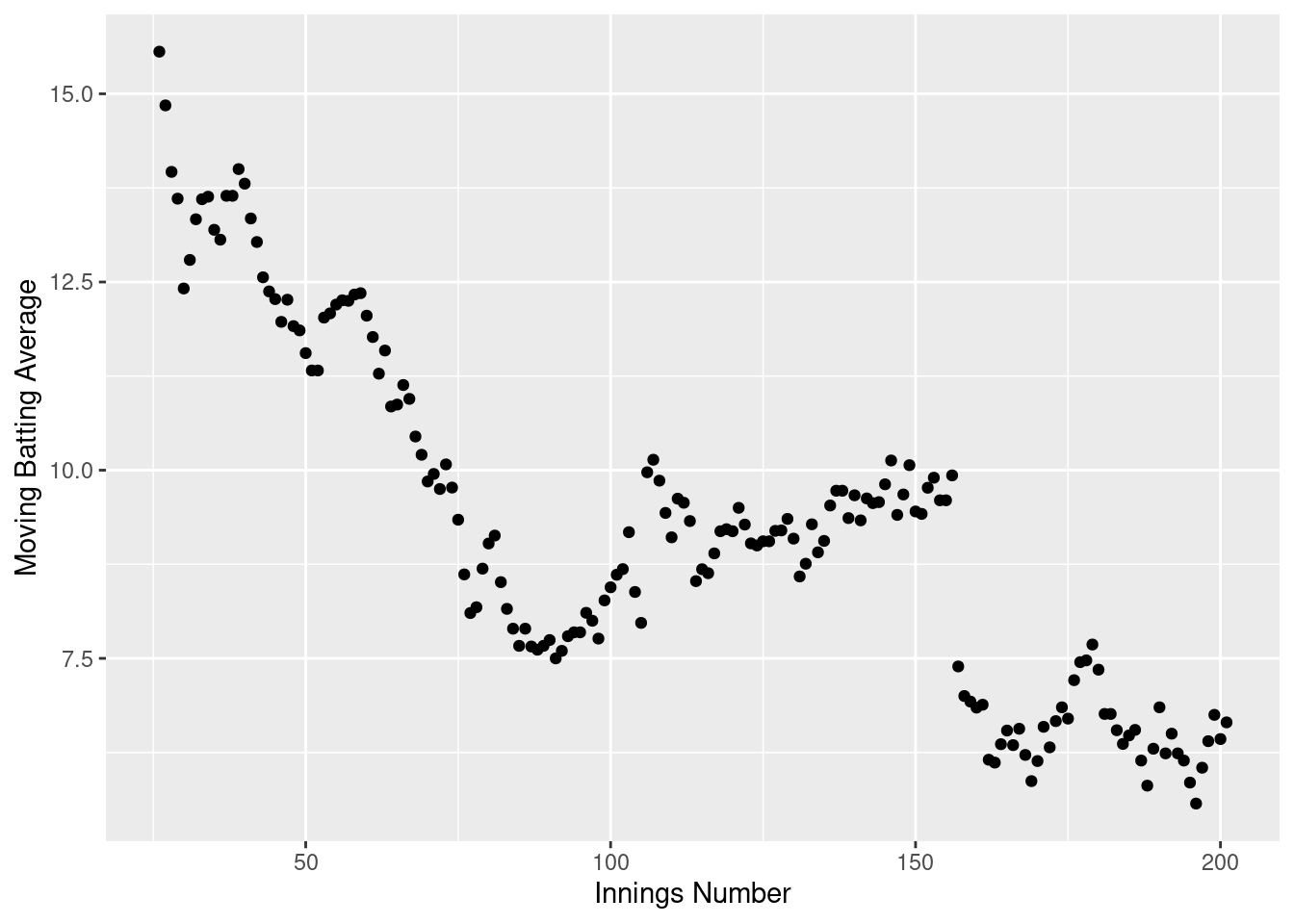
We can see that Jimmy Anderson’s moving batting average has decreased quite a bit from when he started, from ~15 when he began his career to ~6 currently. We can see that this has mostly followed a decreasing shape for his whole career - the only exception being a slight increase in the mid part of his career, which was mostly fuelled by that 81 he scored.
Mathematics
In order to provide an in depth analysis of Jimmy’s batting over time, I think it is necessary to construct a model of his batting performance over time. I will make a fairly simple model by assuming that the runs scored comes from a geometric distribution. As I have previously said, we have to make the following two assumptions:
- If you are not dismissed before scoring another run then you score one extra run.
- The probability of being dismissed before scoring another run is constant, for a given time \(t\).
It is clear that assumption (i) is false and the data is not generated this way because of the rules of cricket, and therefore a more sophisticated model would take this into account and model the underlying process more carefully. The second assumption is also probably false - batting in cricket becomes a lot easier after you have faced a number of deliveries because you have got more used to the bowlers and the conditions.
We also have to deal with times where he is not dismissed. We can think of these times as a censored observation - the innings ended and therefore we don’t know what score he would have ended up on, but we know he would have scored at least the score that he was on at the time.
So mathematically speaking, we will design out model as follows:
\[ \alpha_{i} \sim Geom(\theta_{t[i]}) \\ score_{i} = \begin{cases} \alpha_{i}, \text{if dismissed}, \\ \{0, \dots, \alpha_{i}\}, \text{if not dismissed} \end{cases} \]
Modelling
To start off with our model, I will define some cut off points for our training set (and also the warm up for the exponential weighted model below):
warm_up_cut_off_year <- 2009
train_cut_off_year <- 2016
Exponential Weighted Moving Average
The first model that I will construct will be an exponential weighted moving mean. I will take each timestep as an individual innings, and optimize the weight such that the log likelihood is maximised. I do this in a slightly weird way where I recalculate the weighting parameter for each new observation in the test set - the reason I do this becomes clearer once I describe the state space model below.
source("src/exponential_weighted_moving_average.R")

warm_up_cut_off_year <- 2009
train_cut_off_year <- 2016

warm_up_cut_off <- batting %>%
  filter(year(date) <= warm_up_cut_off_year) %>%
  nrow

train_cut_off <- batting %>%
  filter(year(date) <= train_cut_off_year) %>%
  nrow

weights <- numeric(nrow(batting))
for (i in (train_cut_off+1):nrow(batting)) {
  train <- batting %>%
    filter(innings_no < i)
  weights[i] <- get_optimal_weight(
    warm_up_cut_off,
    train$innings_no,
    train$score,
    !train$dismissed
  )
}

print(paste0("The optimal weight is: ", weights[nrow(batting)]))
[1] "The optimal weight is: 0.0157578544617485"We can now use our calculated weights for each time point to calculate our predicted parameters for the test set, which we will then plot:
params_by_timestep <- numeric(nrow(batting))
for (i in (train_cut_off+1):nrow(batting)) {
  params_by_timestep[i] <- get_params_by_timestep(
    weights[i],
    warm_up_cut_off = warm_up_cut_off,
    timestep_vec = batting$innings_no,
    score_vec = batting$score,
    not_out_vec = !batting$dismissed
  )[i]
}

weighted_moving_ave_preds_by_innings_df <- tibble(
  innings_no  = 1:max(batting$innings_no),
  param = params_by_timestep
) %>%
  filter(innings_no > train_cut_off)

weighted_moving_ave_preds_by_innings_df %>%
  ggplot(aes(x = innings_no, y = param)) +
  geom_point() +
  scale_x_continuous(name = "Innings Number") +
  scale_y_continuous(name = "Parameter")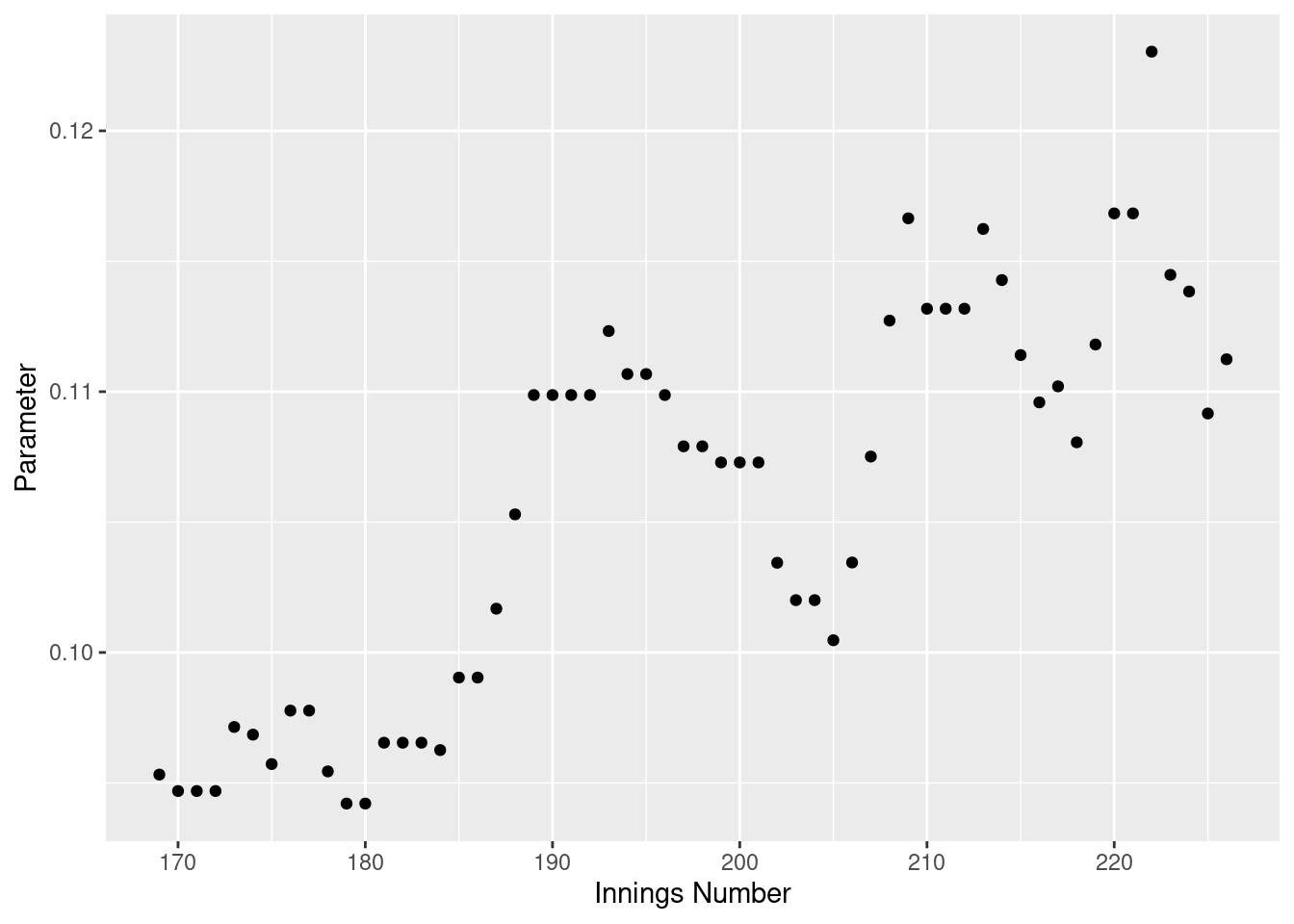
I will now construct a model in the same way as above, but instead of taking each timestep as an individual innings, I will only take the timesteps as individual years.
weights <- numeric(max(year(batting$date)))
for (i in (train_cut_off_year+1):max(year(batting$date))) {
  train <- batting %>%
    filter(year(date) < i)
  weights[i] <- get_optimal_weight(
    warm_up_cut_off_year,
    year(train$date),
    train$score,
    !train$dismissed
  )
}

print(paste0("The optimal weight is: ", weights[i]))
[1] "The optimal weight is: 0.268949564172078"And lets again calculate our predicted parameters for the test set:
params_by_timestep <- numeric(nrow(batting))
for (i in (train_cut_off_year+1):max(year(batting$date))) {
  params_by_timestep[i] <- get_params_by_timestep(
    weights[i],
    warm_up_cut_off = warm_up_cut_off_year,
    timestep_vec = year(batting$date),
    score_vec = batting$score,
    not_out_vec = !batting$dismissed
  )[i]
}

weighted_moving_ave_preds_by_year_df <- tibble(
  year  = 1:max(year(batting$date)),
  param = params_by_timestep
) %>%
  filter(year > train_cut_off_year)

weighted_moving_ave_preds_by_year_df %>%
  ggplot(aes(x = year, y = param)) +
  geom_point() +
  scale_x_continuous(name = "Year") +
  scale_y_continuous(name = "Parameter")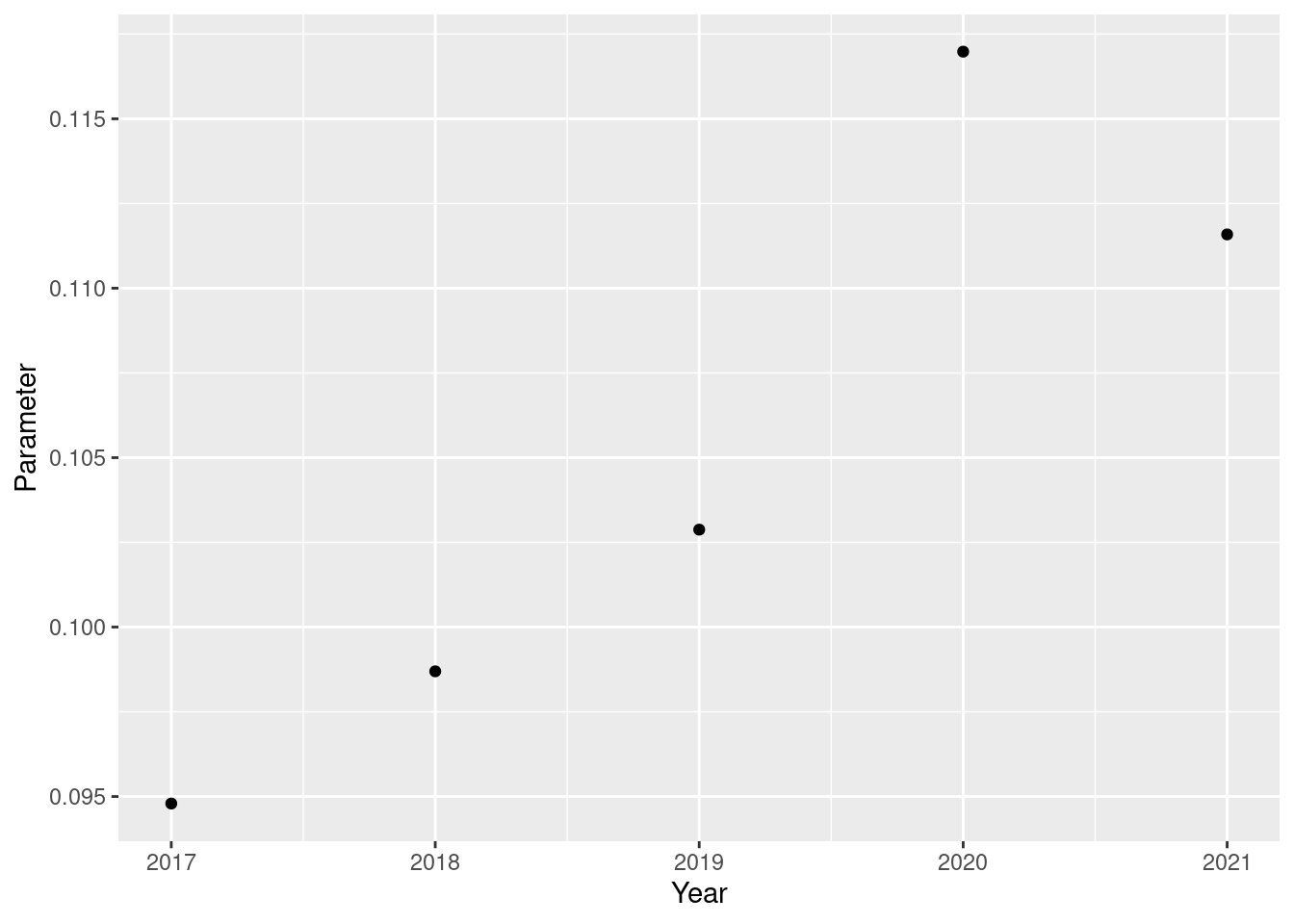
State Space Model
I will now construct a different type of time series model, called a state space model. We will let the parameter of the geometric distribution be the state, and then let this value evolve over time. We will let the state evolve through the equation \(\theta_{t+1} \sim \mathcal{N(\theta_{t}, \sigma)}\).
I have written this model in a language called Stan, a probabilistic programming language for statistical inference. I display the model below.
writeLines(readLines("stan_models/model.stan"))functions {
real geometric_lpmf(int y, real theta) {
return log(theta) + y * log(1 - theta);
}
real geometric_lccdf(int y, real theta) {
return (y + 1) * log(1 - theta);
}
}
data {
int<lower=1> num_outs;
int<lower=1> num_not_outs;
int<lower=1> ntimesteps;
int<lower=1, upper=ntimesteps> timestep_out[num_outs];
int<lower=1, upper=ntimesteps> timestep_not_out[num_not_outs];
int<lower=0> score_out[num_outs];
int<lower=0> score_not_out[num_not_outs];
}
parameters {
real initial_param;
real unscaled_param[ntimesteps-1];
real<lower=0> sigma;
}
transformed parameters {
real param[ntimesteps];
real transformed_param[ntimesteps];
param[1] = initial_param;
for (k in 2:ntimesteps) {
param[k] = param[k-1] + unscaled_param[k-1] * sigma;
}
transformed_param = inv_logit(param);
}
model {
for (i in 1:num_outs) {
target += geometric_lpmf(score_out[i] | transformed_param[timestep_out[i]]);
}
for (i in 1:num_not_outs) {
target += geometric_lccdf( (score_not_out[i] - 1) | transformed_param[timestep_not_out[i]]);
}
initial_param ~ normal(-2.25, 0.5);
unscaled_param ~ std_normal();
sigma ~ std_normal();
}Now, it can be difficult to fit a state space model with too many parameters, so I will only run this model where each timestep is a year. Below I load in the model and do statistical inference.
model <- stan_model("stan_models/model.stan")hash mismatch so recompiling; make sure Stan code ends with a blank linetrain <- batting %>%
filter(year(date) <= train_cut_off_year)
standata <- list(
num_outs = sum(train$dismissed),
num_not_outs = sum(!train$dismissed),
ntimesteps = max(year(train$date)) - 2002,
timestep_out = year(train$date[train$dismissed]) - 2002,
timestep_not_out = year(train$date[!train$dismissed]) - 2002,
score_out = train$score[train$dismissed],
score_not_out = train$score[!train$dismissed]
)
fit <- sampling(model, standata, seed = 1, iter = 10000, control = list(adapt_delta = 0.995))The first thing to do after MCMC is to check the fit. Let’s start by printing the output of the fit.
print(fit)Inference for Stan model: anon_model.
4 chains, each with iter=10000; warmup=5000; thin=1;
post-warmup draws per chain=5000, total post-warmup draws=20000.
mean se_mean sd 2.5% 25% 50% 75%
initial_param -2.48 0.00 0.26 -3.07 -2.64 -2.46 -2.31
unscaled_param[1] 0.08 0.01 0.93 -1.75 -0.54 0.08 0.71
unscaled_param[2] 0.08 0.01 0.94 -1.78 -0.55 0.07 0.70
unscaled_param[3] 0.10 0.01 0.93 -1.72 -0.52 0.09 0.73
unscaled_param[4] 0.00 0.01 0.91 -1.79 -0.60 0.00 0.62
unscaled_param[5] -0.30 0.01 0.93 -2.06 -0.94 -0.33 0.31
unscaled_param[6] 0.36 0.01 0.88 -1.37 -0.22 0.36 0.93
unscaled_param[7] 0.87 0.01 0.92 -1.03 0.29 0.90 1.49
unscaled_param[8] -0.06 0.01 0.93 -1.79 -0.70 -0.09 0.56
unscaled_param[9] 0.25 0.01 0.87 -1.47 -0.31 0.25 0.83
unscaled_param[10] 0.00 0.01 0.86 -1.66 -0.57 -0.01 0.56
unscaled_param[11] -0.28 0.01 0.88 -1.91 -0.88 -0.31 0.29
unscaled_param[12] 0.50 0.01 0.90 -1.38 -0.08 0.53 1.10
unscaled_param[13] 0.02 0.01 0.91 -1.77 -0.59 0.01 0.63
sigma 0.20 0.00 0.16 0.01 0.08 0.16 0.28
param[1] -2.48 0.00 0.26 -3.07 -2.64 -2.46 -2.31
param[2] -2.46 0.00 0.27 -3.06 -2.61 -2.44 -2.29
param[3] -2.45 0.00 0.29 -3.09 -2.60 -2.42 -2.28
param[4] -2.42 0.00 0.25 -2.97 -2.57 -2.41 -2.27
param[5] -2.43 0.00 0.23 -2.92 -2.55 -2.41 -2.29
param[6] -2.52 0.00 0.23 -3.08 -2.65 -2.49 -2.36
param[7] -2.45 0.00 0.19 -2.87 -2.55 -2.42 -2.32
param[8] -2.23 0.00 0.22 -2.59 -2.38 -2.26 -2.13
param[9] -2.29 0.00 0.19 -2.68 -2.40 -2.29 -2.17
param[10] -2.23 0.00 0.17 -2.55 -2.35 -2.24 -2.13
param[11] -2.24 0.00 0.17 -2.56 -2.35 -2.25 -2.14
param[12] -2.33 0.00 0.19 -2.76 -2.43 -2.31 -2.21
param[13] -2.20 0.00 0.20 -2.56 -2.33 -2.22 -2.08
param[14] -2.20 0.00 0.23 -2.63 -2.35 -2.22 -2.06
transformed_param[1] 0.08 0.00 0.02 0.04 0.07 0.08 0.09
transformed_param[2] 0.08 0.00 0.02 0.04 0.07 0.08 0.09
transformed_param[3] 0.08 0.00 0.02 0.04 0.07 0.08 0.09
transformed_param[4] 0.08 0.00 0.02 0.05 0.07 0.08 0.09
transformed_param[5] 0.08 0.00 0.02 0.05 0.07 0.08 0.09
transformed_param[6] 0.08 0.00 0.02 0.04 0.07 0.08 0.09
transformed_param[7] 0.08 0.00 0.01 0.05 0.07 0.08 0.09
transformed_param[8] 0.10 0.00 0.02 0.07 0.08 0.09 0.11
transformed_param[9] 0.09 0.00 0.02 0.06 0.08 0.09 0.10
transformed_param[10] 0.10 0.00 0.02 0.07 0.09 0.10 0.11
transformed_param[11] 0.10 0.00 0.02 0.07 0.09 0.10 0.11
transformed_param[12] 0.09 0.00 0.01 0.06 0.08 0.09 0.10
transformed_param[13] 0.10 0.00 0.02 0.07 0.09 0.10 0.11
transformed_param[14] 0.10 0.00 0.02 0.07 0.09 0.10 0.11
lp__ -367.95 0.06 3.59 -375.46 -370.24 -367.80 -365.49
97.5% n_eff Rhat
initial_param -2.02 12192 1
unscaled_param[1] 1.90 21408 1
unscaled_param[2] 1.94 22661 1
unscaled_param[3] 1.94 21908 1
unscaled_param[4] 1.82 23783 1
unscaled_param[5] 1.57 18775 1
unscaled_param[6] 2.09 22763 1
unscaled_param[7] 2.59 15050 1
unscaled_param[8] 1.85 16593 1
unscaled_param[9] 1.96 22638 1
unscaled_param[10] 1.73 23524 1
unscaled_param[11] 1.55 19090 1
unscaled_param[12] 2.21 17907 1
unscaled_param[13] 1.85 24889 1
sigma 0.61 5534 1
param[1] -2.02 12192 1
param[2] -1.95 19298 1
param[3] -1.89 19299 1
param[4] -1.93 23715 1
param[5] -2.00 22523 1
param[6] -2.16 10851 1
param[7] -2.13 15148 1
param[8] -1.71 11187 1
param[9] -1.89 21349 1
param[10] -1.86 17812 1
param[11] -1.88 19119 1
param[12] -2.00 18853 1
param[13] -1.76 14021 1
param[14] -1.71 18471 1
transformed_param[1] 0.12 12966 1
transformed_param[2] 0.12 20119 1
transformed_param[3] 0.13 19828 1
transformed_param[4] 0.13 23666 1
transformed_param[5] 0.12 22634 1
transformed_param[6] 0.10 10415 1
transformed_param[7] 0.11 14900 1
transformed_param[8] 0.15 11247 1
transformed_param[9] 0.13 21272 1
transformed_param[10] 0.13 17920 1
transformed_param[11] 0.13 19189 1
transformed_param[12] 0.12 19046 1
transformed_param[13] 0.15 14017 1
transformed_param[14] 0.15 18314 1
lp__ -361.29 4160 1
Samples were drawn using NUTS(diag_e) at Tue May 21 14:11:04 2024.
For each parameter, n_eff is a crude measure of effective sample size,
and Rhat is the potential scale reduction factor on split chains (at
convergence, Rhat=1).So the Rhat value is 1 for everything, which should mean that the chains are well mixed. We can see that the effective sample size is lowest for the sigma parameter. Let’s take a look at the traceplot for this and a few other parameters, just to check that the model has fit okay.
traceplot(fit, "sigma")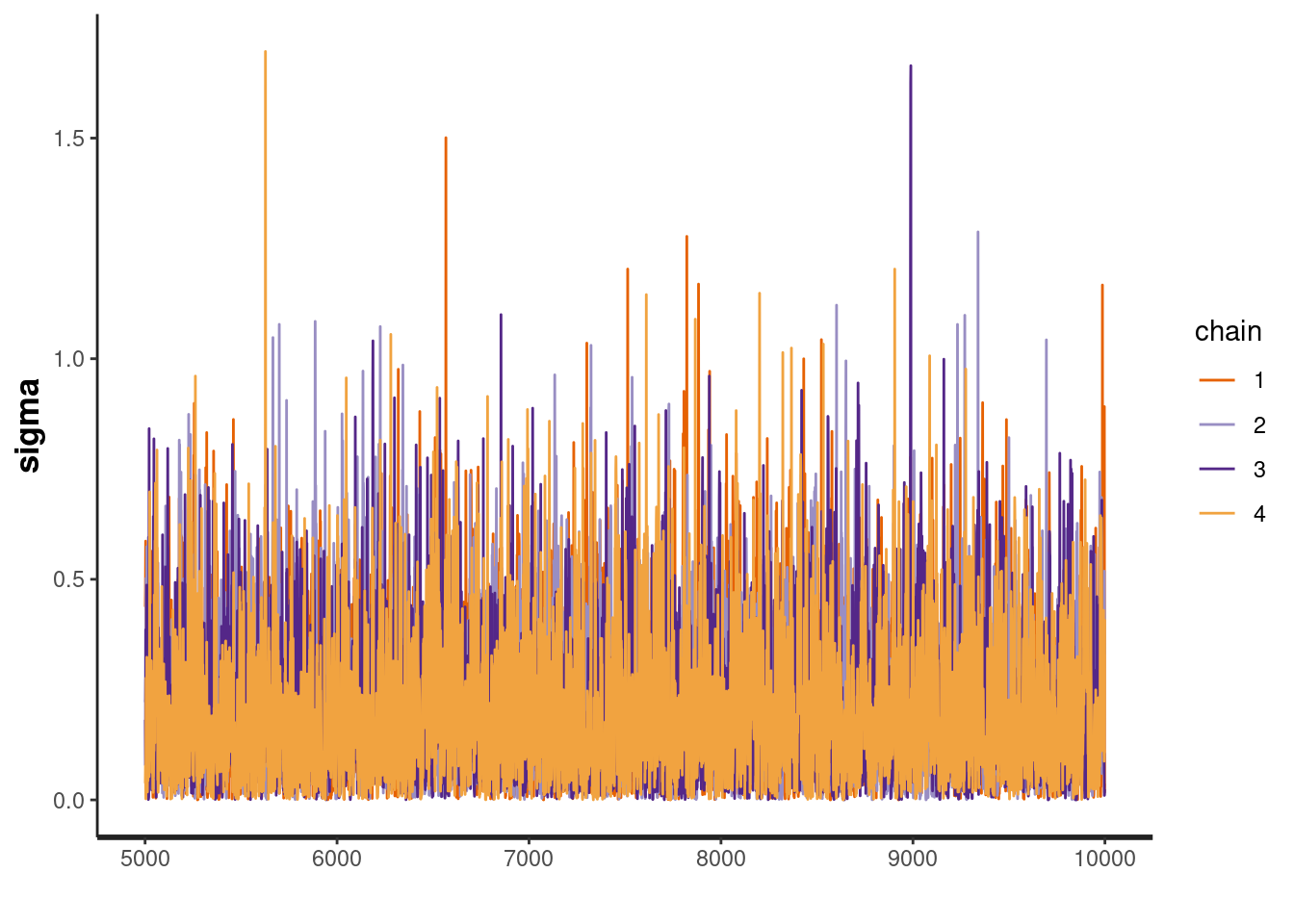
traceplot(fit, "initial_param")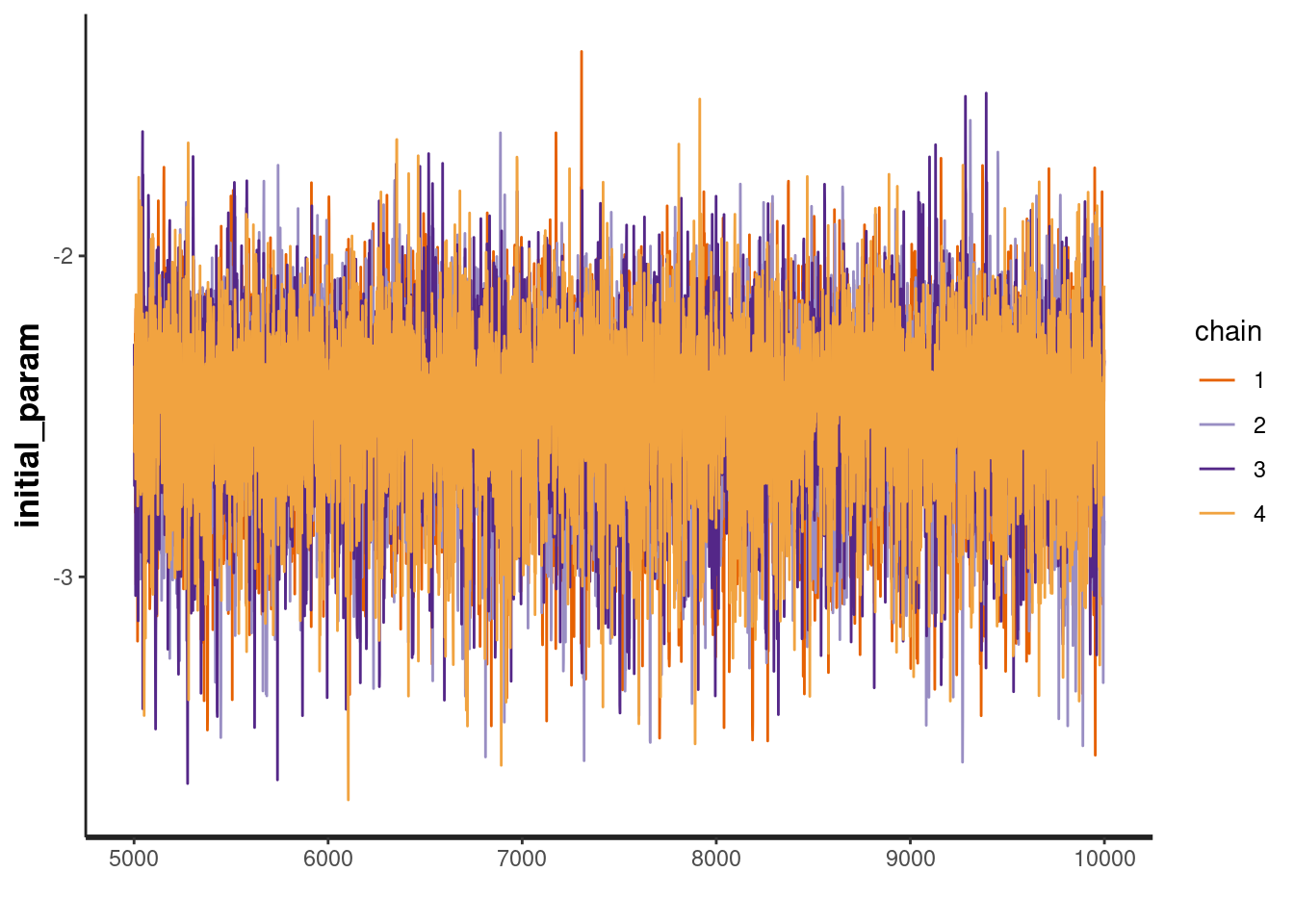
traceplot(fit, "unscaled_param[1]")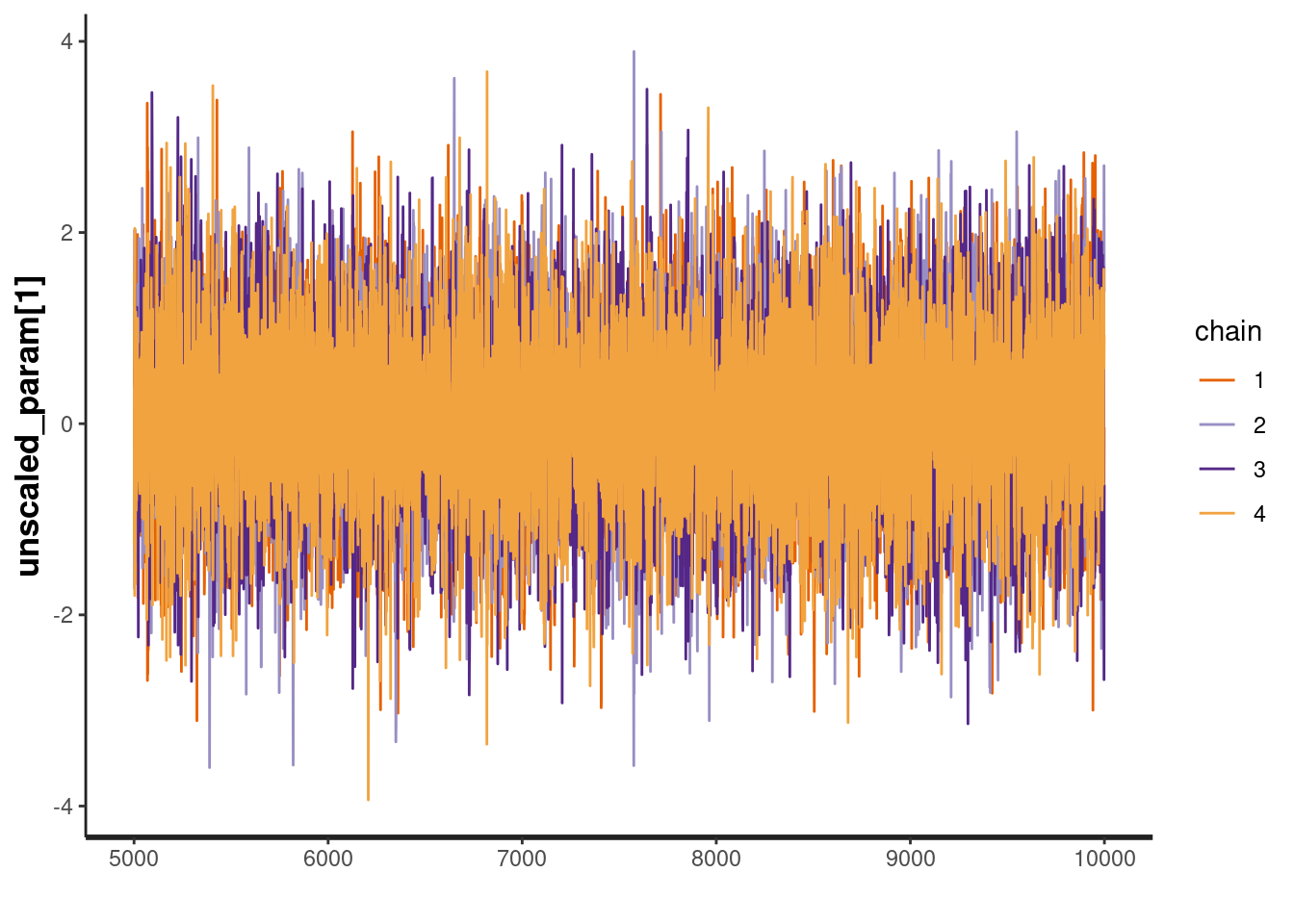
The traceplot for all these parameters look good and the chains are well mixed. Therefore we can conclude that our chains have probably converged.
We now want to calculate our predicted parameters for each year. To do this, we need to retrain the model for each year with the updated dataset (a technique called filtering is often used to do this instead of retraining the model).
fits <- list()
for (i in (train_cut_off_year+1):max(year(batting$date))) {
  train <- batting %>%
    filter(year(date) < i)
  standata <- list(
    num_outs = sum(train$dismissed),
    num_not_outs = sum(!train$dismissed),
    ntimesteps = max(year(train$date)) - 2002,
    timestep_out = year(train$date[train$dismissed]) - 2002,
    timestep_not_out = year(train$date[!train$dismissed]) - 2002,
    score_out = train$score[train$dismissed],
    score_not_out = train$score[!train$dismissed]
  )
  fits[[as.character(i)]] <- sampling(
    model,
    standata,
    seed = 1,
    iter = 10000,
    control = list(adapt_delta = 0.995),
    open_progress = FALSE,
    show_messages = FALSE,
    refresh = -1
  )
}
Since we have refitted the models on each extra bit of training data, we now have our predicted parameters. Lets plot them to see what they look like.
params_by_timestep <- numeric(nrow(batting))
for (i in (train_cut_off_year+1):max(year(batting$date))) {
  params_by_timestep[i] <- extract(fits[[as.character(i)]])[["transformed_param"]][,i-2003] %>% mean
}

state_space_preds_df <- tibble(
  year  = 1:max(year(batting$date)),
  param = params_by_timestep
) %>%
  filter(year > train_cut_off_year)

state_space_preds_df %>%
  ggplot(aes(x = year, y = param)) +
  geom_point() +
  scale_x_continuous(name = "Year") +
  scale_y_continuous(name = "Parameter")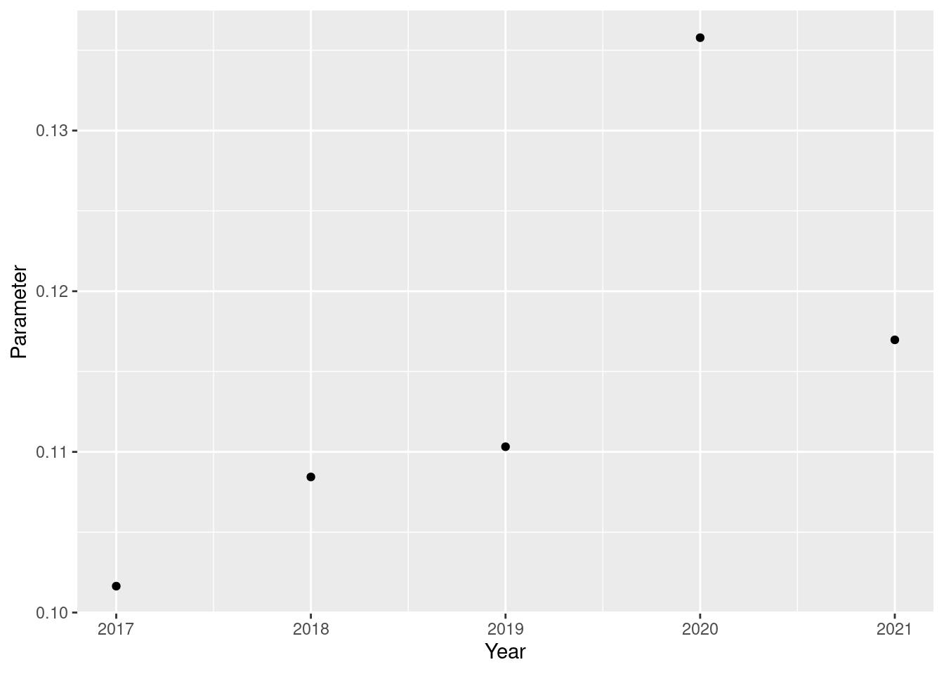
Model Comparison
Now that I have predicted parameters from all the models, I can calculate their log loss scores and compare them.
test <- batting %>%
  filter(year(date) > train_cut_off_year)

weighted_mov_ave_preds_by_innings <- numeric(nrow(test))
weighted_mov_ave_preds_by_year <- numeric(nrow(test))
state_space_preds <- numeric(nrow(test))

for (i in 1:nrow(test)) {
  weighted_mov_ave_preds_by_innings[i] <- weighted_moving_ave_preds_by_innings_df %>%
    filter(innings_no == test$innings_no[i]) %>%
    pull(param)
  weighted_mov_ave_preds_by_year[i] <- weighted_moving_ave_preds_by_year_df %>%
    filter(year == year(test$date[i])) %>%
    pull(param)
  state_space_preds[i] <- state_space_preds_df %>%
    filter(year == year(test$date[i])) %>%
    pull(param)
}

print(get_neg_log_lik(weighted_mov_ave_preds_by_innings, test$score, !test$dismissed))
[1] 69.13824print(get_neg_log_lik(weighted_mov_ave_preds_by_year, test$score, !test$dismissed))[1] 68.97544print(get_neg_log_lik(state_space_preds, test$score, !test$dismissed))[1] 68.76052So we can see that the state space model gives us the best predictions on this test set.
Future Work
A few improvements that could be done for this model in the future:
- Address assumption (i) - a possible way of doing this is to model the number of balls faced as an intermediate step, and then runs scored from this.
- Address assumption (ii) by assuming that the probability of being dismissed changes as his innings progresses.
- Include other key factors such as the strength of the opposition and the match conditions.
Conclusion
Lets take our best model and look at what it says about Jimmy Anderson’s batting strength over time:
standata <- list(
  num_outs = sum(batting$dismissed),
  num_not_outs = sum(!batting$dismissed),
  ntimesteps = max(year(batting$date)) - 2002,
  timestep_out = year(batting$date[batting$dismissed]) - 2002,
  timestep_not_out = year(batting$date[!batting$dismissed]) - 2002,
  score_out = batting$score[batting$dismissed],
  score_not_out = batting$score[!batting$dismissed]
)

fit <- sampling(
  model,
  standata,
  seed = 1,
  iter = 10000,
  control = list(adapt_delta = 0.995),
  open_progress = FALSE,
  show_messages = FALSE,
  refresh = -1
)

params_by_timestep <- numeric(nrow(batting)+1)
model_params <- extract(fit)
for (i in 2004:2022) {
  params_by_timestep[i] <- mean(model_params[["transformed_param"]][,i-2003])
}

state_space_preds_df <- tibble(
  year  = 1:(max(year(batting$date))+1),
  param = params_by_timestep
) %>%
  filter(year > 2003) %>%
  mutate(exp_ave = (1 - param) / param)

state_space_preds_df %>%
  ggplot(aes(x = year, y = exp_ave)) +
  geom_point() +
  scale_x_continuous(name = "Year") +
  scale_y_continuous(name = "Parameter", limits = c(7, 12))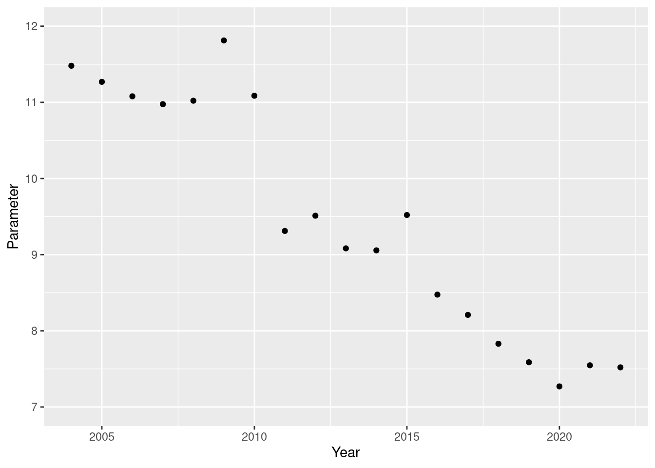
In conclusion, the two things that stand out to me are:
- It seems to show that from 2010 Jimmy’s batting got a lot worse - it would be interesting to know what caused quite a large and sudden change.
- His batting has undergone a steady decline towards the back end of his career, as is often said by commentators and pundits.